Bicing Prediction Models with Machine Learning

A scrollytelling case study on forecasting bike availability across Barcelona’s Bicing network using temporal filtering, feature engineering, and tree-based ensemble models.

The prototype learned the broad rhythm of the system, but it also exposed the harder truth: bike-share prediction is a spatial rebalancing problem, not just a tabular regression task.

Training window 2021–2023 only
Best unseen score GBR · 0.074 MSE
Core challenge Spatial demand shifts
Scroll to enter the system
Narrative Audit

From hourly bike counts to a city-scale forecasting problem.

This project set out to predict the proportional availability of bikes at any Bicing station at any hour in Q1 2024. What begins as a machine learning exercise quickly becomes an urban systems problem: demand shifts uphill and downhill, anomalous years distort the training distribution, and not every feature that seems intuitive actually carries predictive value.
Signal Matrix

Not all theoretically useful features become operationally useful.

The source article frames the feature set as a tension between intuition and actual model utility. Time was the strongest signal, spatial context was under-specified, and temperature alone was too weak to stand in for weather-driven suppression.

Category Features Expected role Observed utility
Spatial Latitude, longitude, altitude Capture slope & neighborhood context Useful, but incomplete without spatial lag
Temporal Hour, day type, month Encode commuting & leisure cycles Strongest predictive signal
Meteorological Hourly temperature Approximate weather deterrence Weak proxy without rain, wind, humidity
Demand context Capacity, population density Represent supply pressure & local demand Moderate, but still blunt
Act I

The System Problem

Forecasting bike availability is not just about one station at one hour. It is about how flows move across a network shaped by commute cycles, topography, and neighborhood asymmetry.

Context & Problem Definition

Bicing availability behaves like an uneven urban field.

Barcelona’s bike-share network spans flat central districts and steeper uphill neighborhoods. That means bikes do not simply appear and disappear randomly; they drain downhill during commute cycles and empty faster uphill, making rebalancing a spatial systems issue.

  • Downhill stations accumulate bikes; uphill stations empty early.
  • Station behavior depends on neighboring stations and city topography.
Target variable

The model predicts proportional availability, not raw bike counts.

Normalizing available bikes by station capacity lets the prediction target stay comparable across the network. That choice makes the output operationally meaningful, but it also raises the bar for the input features: simple tabular signals are not enough to explain the dynamics by themselves.

15–30
Minutes of app forecast is not enough for cross-city planning.

The original problem statement is strategic: a rider needs more than a short forecast window when station availability depends on wider urban flows.

Act II

Audit the Training Window

Before model selection, the project had to answer a more important question: which years still describe the world the model will be deployed into?

Temporal filtering

The most consequential model decision happened before training.

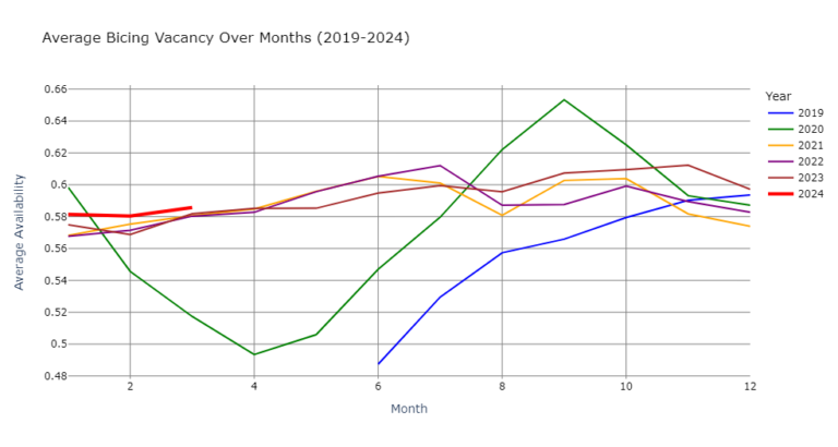
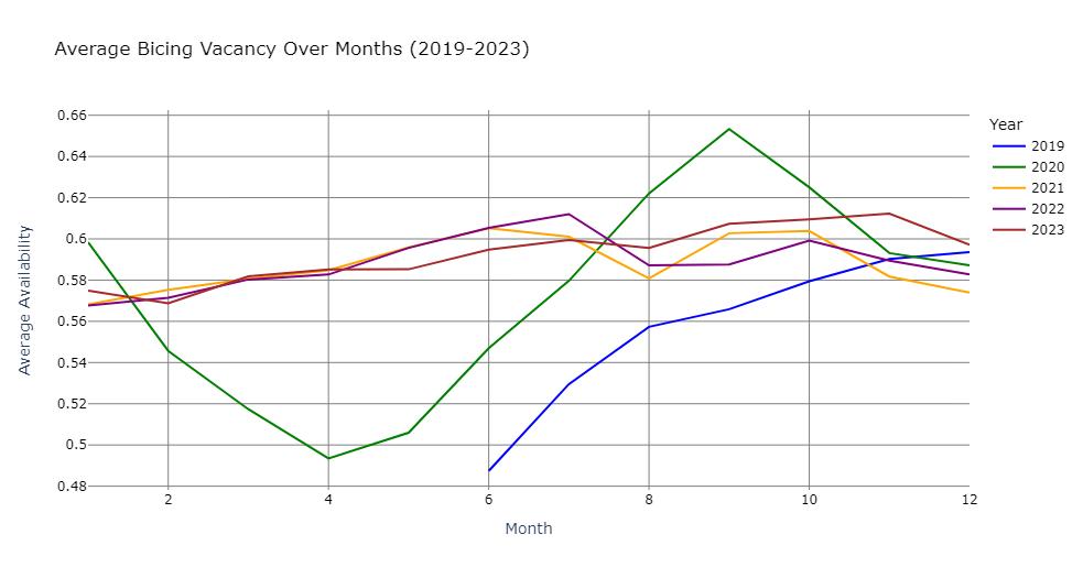
The longitudinal availability plot showed two structural breaks: the Bicing 2.0 platform rollout in 2019 and the COVID demand shock in 2020. Including those periods would have polluted the training distribution with behavior that no longer matched the deployment environment.

Regime change

2019 and 2020 are not noisy years; they are different systems.

2019 reflects transition noise from the Bicing 2.0 launch. 2020 reflects a lockdown collapse and anomalous rebound. Training on both would teach the model that those distorted availability baselines are normal.

  • 2019: product and reporting instability.
  • 2020: demand shock and rebound, not steady-state mobility.
Weather signal

Temperature alone is an intuitive feature, but a weak operational one.

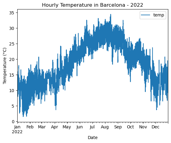
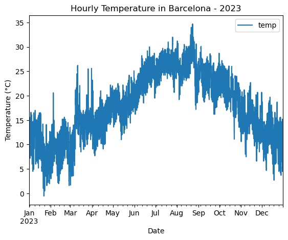
The project sourced hourly temperature, but Barcelona’s cycling suppression is more tightly coupled to intense rain events than to winter cold. The weather charts help explain why the meteorological channel stayed weaker than expected.

2021–2023
Three stable years became the final training window.

That choice preserved seasonality and public-holiday variation while avoiding regime-change periods that would bias the model away from current operations.

Act III

Design the Signal, Compare the Models

Once the training window is stable, the story shifts to signal design: which features genuinely explain bike availability, and which model family handles those relationships best?

Population signal

Absolute counts hide the intensity of demand.

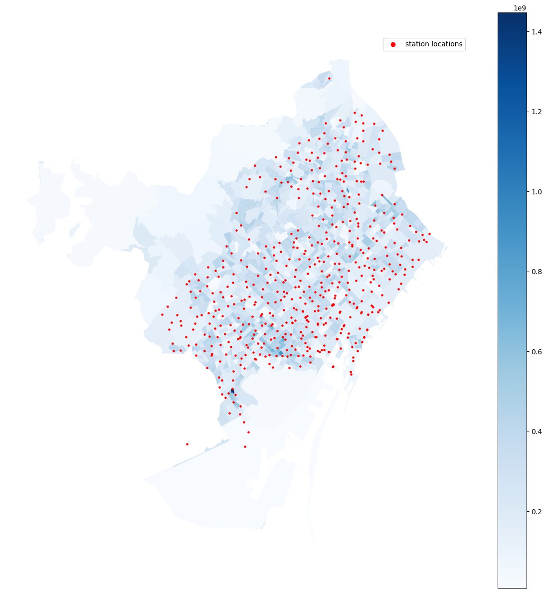
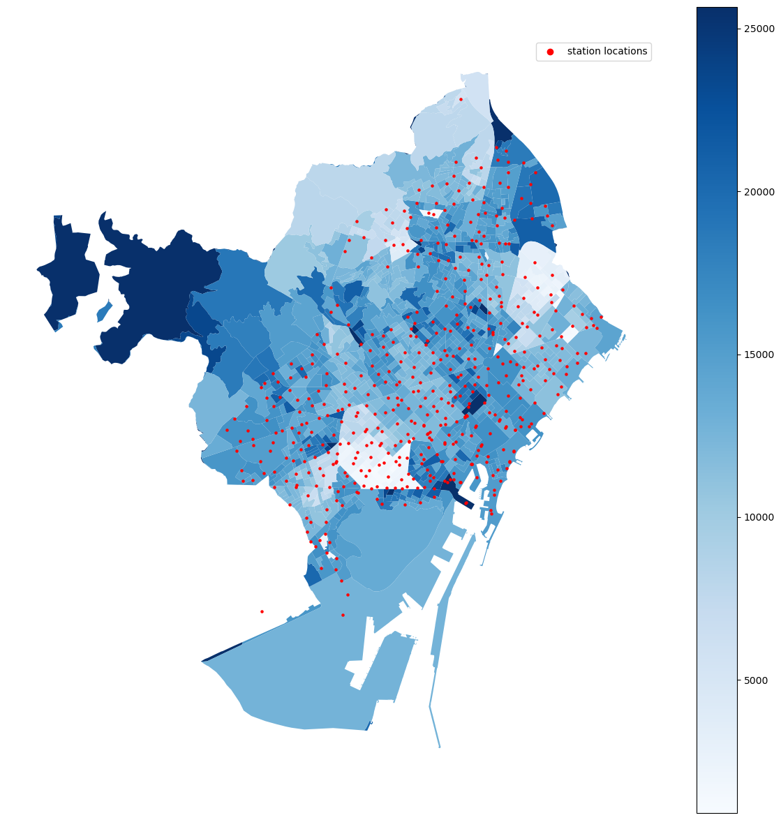
Larger districts dominate raw population totals simply because they cover more area. That makes absolute counts a misleading proxy for bike-share demand. The original article correctly reframes this as a density problem.

Density-normalised input

Population per km² is more useful, but still too blunt on its own.

Density improves the demand proxy, but the article’s own diagnosis is sharper: a POI density score or neighborhood attractor index would explain cycling demand better than residential density alone.

  • Demand depends on offices, schools, universities, and transit nodes.
  • Raw lat/lon still cannot encode neighborhood spillovers explicitly.
Model 1

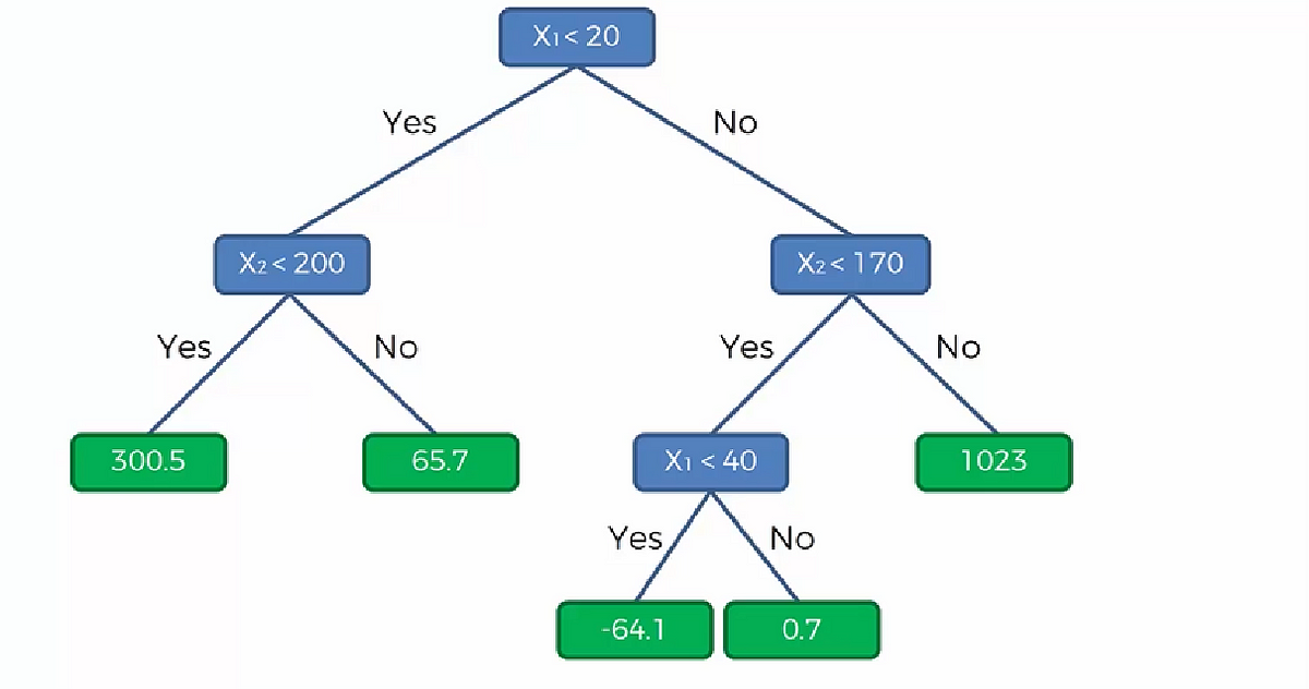
Decision trees are interpretable, but fragile without constraints.

A single decision tree fits the local structure quickly, which makes it useful for inspection. It also makes it easy to overfit discontinuities in training data when the feature set still contains noise.

Model 2

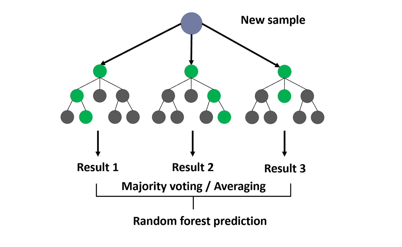
Random forests lowered training error, but not for the right reason.

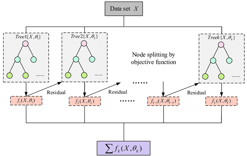
Averaging many decorrelated trees reduces variance inside the training distribution. But the article’s key lesson is that lower training MSE is not proof of better learning when the deployment period is structurally different from the memorized patterns.

0.074
Gradient boosting generalized best on unseen 2024 data.

It was not the most optimistic model on the training set. It was the one that stayed closer to the shape of the real signal once the project crossed into an unseen quarter.

Slide Deck Appendix

Keep the implementation layer visible, but out of the main story.

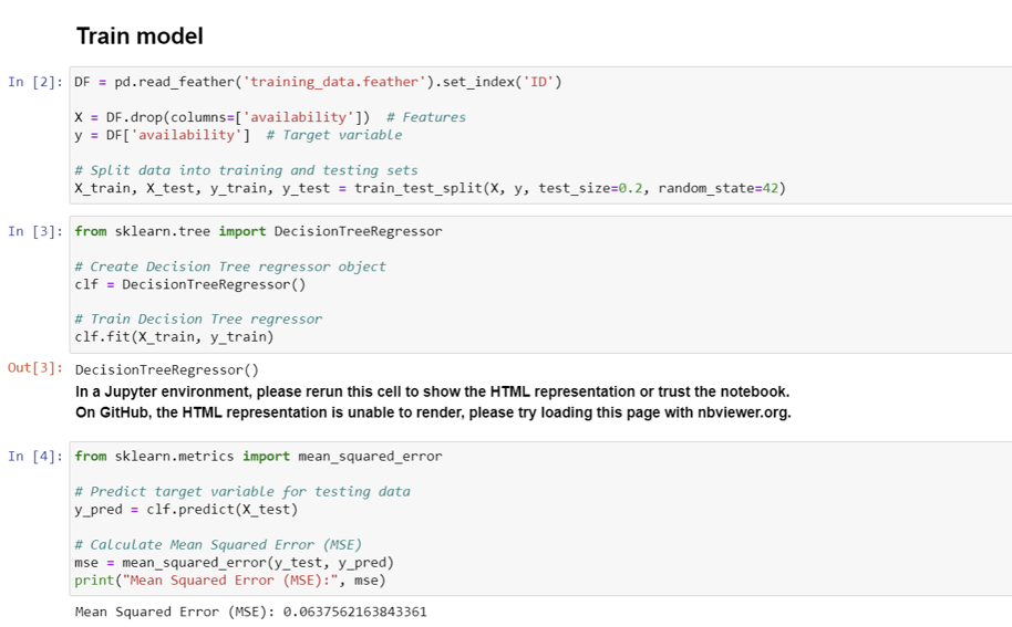
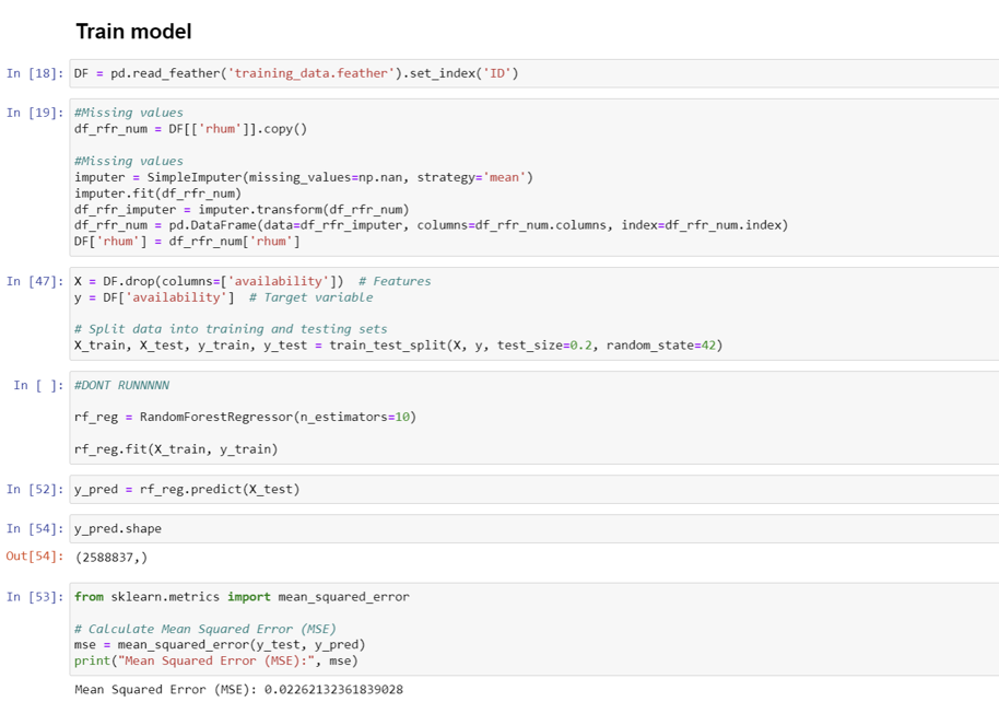
The PDF deck included code-level screenshots for the prototype models. They are useful as supporting evidence of how the classifiers were trained, but not strong enough to carry a full scrollytelling act on their own.

Decision tree training code snippet from the Bicing project slide deck
Decision Tree prototype snippet

Useful as appendix material because it grounds the narrative in an actual training workflow without interrupting the higher-level comparison of signal design and model behavior.

Random forest regressor training code snippet from the Bicing project slide deck
Random Forest prototype snippet

Kept as supporting reference from the slide deck: informative for process context, secondary to the stronger visual evidence in the audit, feature, and diagnosis acts.

Act IV

Diagnose the Overfit, Define the Forward Path

The reveal in the results is not just which model won. It is why the best training score was misleading, why the predictions were systematically smoothed, and what a production version would need to do differently.

Results & Diagnosis

The model learned the average rhythm, not the sharp edges of real demand.

The Q1 2024 plot shows the model following broad weekly and seasonal movement while dampening the sharper morning and evening peaks. That smoothing is the visual signature of a system that generalizes some structure but still misses the abrupt transitions that matter most operationally.

Overfitting came from validation, regularization, and signal design together.

The retrospective diagnosis is precise: there was no time-series cross-validation, no explicit regularization target, and too many features that sounded plausible but carried limited generalizable signal.

The missing features were relational, not just additional.

Spatial lag variables, graph encodings of the station network, and richer meteorological features would have made the model more structurally aware. The project’s own critique is that raw coordinates cannot substitute for relationships across the network.

Gradient boosting predictions compared with actual Bicing availability in 2024
Prediction vs actual The model follows the broad trend, but the mismatch around sharper peaks exposes the gap between a useful prototype and a production-grade forecasting system.
Resolution

Three things the project ultimately proves.

The case study matters not because it solved Bicing forecasting completely, but because it made the failure modes legible. That makes the prototype strategically useful: it defines what a stronger mobility model must encode next.

Data window choice is model design.

Regime-change years can corrupt a training distribution before any algorithm touches the data. Auditing the label over time is as important as model tuning.

Feature engineering needs urban logic.

Spatial lag, slope differentials, POI density, rain, and rebalancing events describe the actual system better than raw coordinates or temperature alone.

Production requires network awareness.

A stronger version would move toward graph-based spatiotemporal learning or a richer boosted-tree pipeline with cyclical encoding and continuous retraining.

Bicing Prediction Models with Machine Learning was developed at the Institute for Advanced Architecture of Catalonia in the Master in City & Technology by Sharon Megan Wong, Diederik de Vries, Nupur Sircar, and Siddharth Nambiar during Digital Tools & Big Data III with Andre Resende.

Final Compliance

References and source logic

This version keeps the original Bicing narrative in semantic HTML but restructures it into a Nocturne-style story: system problem, data audit, signal design, model comparison, and forward path. Local assets replace the source page’s remote figures wherever equivalents were available, while the slide-deck code exports are kept as appendix material rather than promoted into the main scroll.

Methodological through-line
  1. Frame Bicing availability as a networked urban systems problem.
  2. Exclude structurally anomalous years before training.
  3. Compare feature utility instead of assuming every plausible variable helps.
  4. Read lower training error skeptically when generalization worsens.
  5. Use the prototype to define the next production architecture.
Local assets used
  1. `Picture1.jpg` and `ML_Algo.png` for the hero and system framing.
  2. `newplot-2.png`, `Hourly_Temp_Data_2022.png`, and `Hourly_Temp_Data_2023.png` for data audit and weather signal discussion.
  3. `Population Data1.png`, `Population_Data2.png`, `Decision_tree.png`, and `Random_Forest.png` for feature and model comparison.
  4. `Decision_Tree_TrainModel_Code_Snippet.png`, `RandomForest_Regressor_Code_Snippet.png`, and `Bicing Prediction_slides.pdf` as supporting implementation references.
  5. `newplot-1-768x410.png` for the final diagnosis and prediction-vs-actual reading.