Panoramic Vision

A computational streetscape analysis that turns panoramic street imagery into an urban reading system: sampling streets, estimating depth, clustering visual patterns, and using those groupings to interpret street quality at city scale.

“Can we understand urban environments and street characteristics from Google Street View panorama images using machine learning and Stable Diffusion techniques?”

Computational design Python + Grasshopper
Street imagery Barcelona panoramas
ML workflow Depth + clustering
Scroll to enter the pipeline
Narrative Audit

From street snapshots to an urban typology.

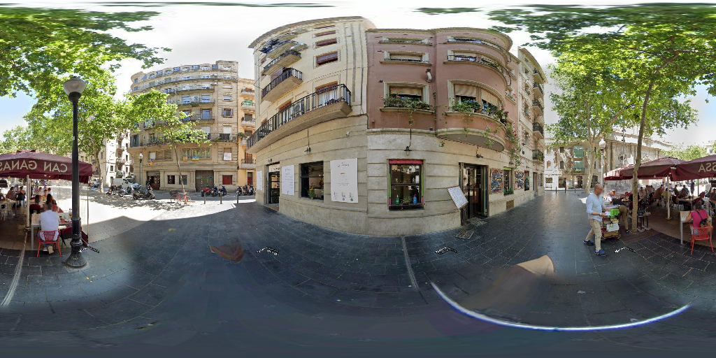
Street quality is often described qualitatively and site by site. This project reframes that task as a repeatable computational pipeline: identify a study area, gather panoramic street views, convert them into depth readings, cluster the resulting patterns, and map those groups back onto the city.

1. Sample Bound the study area, extract street centerlines, and locate panorama capture points.
2. Translate Use Stable Diffusion depth estimation to turn color panoramas into spatial readings.
3. Cluster Reduce dimensionality with t-SNE and compare groups with clustering analysis.
4. Interpret Read distance distributions to infer openness, clutter, edge conditions, and street quality.
Act I

Sampling the street

The first challenge is not analysis but framing: deciding where the city begins for the study, which streets matter, and how each panorama becomes a comparable urban sample.

Structural Mapping

Define the study area before reading the image.

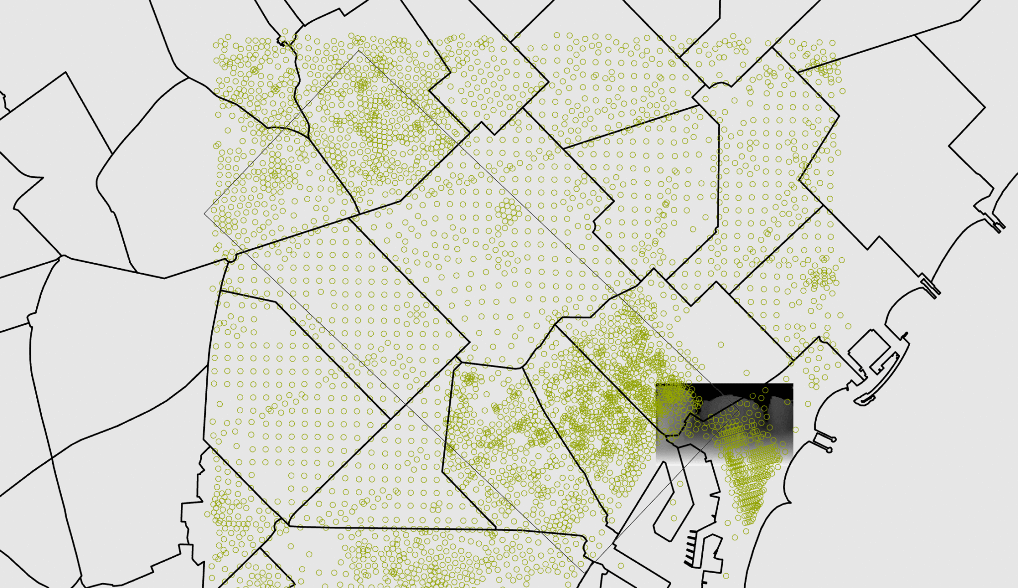
The workflow starts with a Python script that defines the boundary of the site and extracts street center points from OpenStreetMap. Each point becomes a potential panorama sample tied to the street network rather than an isolated picture.

  • Boundary selection anchors the analysis to a precise geographic scope.
  • Street center points become the bridge between GIS geometry and image capture.
Input stack

Three inputs keep the street view pipeline spatially grounded.

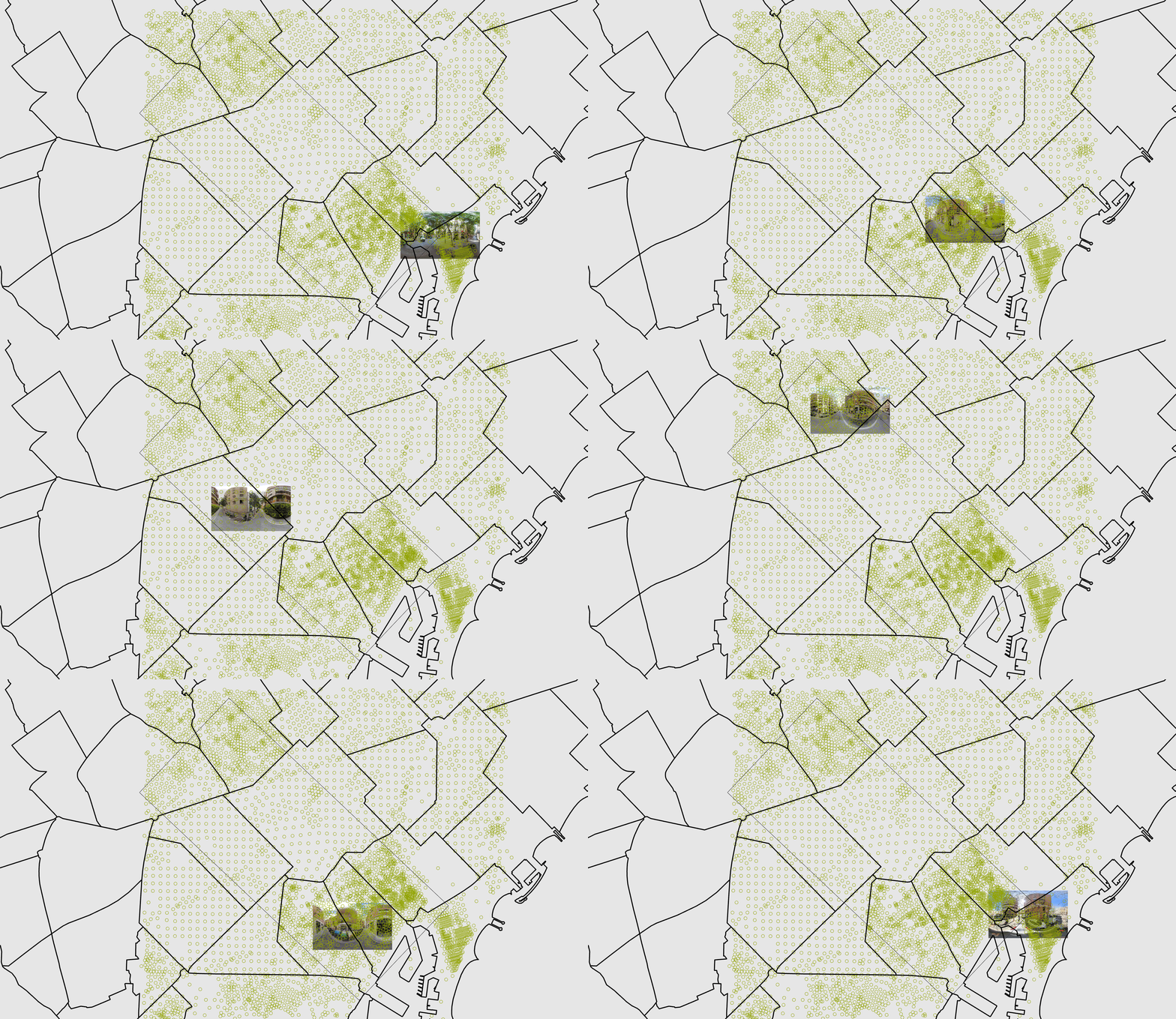
Panorama images, a shapefile of streets, and a coordinate CSV are connected inside Grasshopper. That lets the team crop a target area, review the image coverage, and pass the selected file paths into the next depth-processing step.

  • Panorama filenames preserve traceability between image and location.
  • Street geometry keeps the visual dataset tied to the urban network.
1
One panorama becomes a measurable street section.

Instead of treating imagery as mood-board material, the project treats each panorama as a spatial observation that can be translated, compared, and clustered across the city.

Act II

Translating image into depth

The tension in the workflow is that a panorama is still a flat image. Depth estimation is the moment where the street starts behaving less like a photograph and more like a measurable spatial field.

Methodology

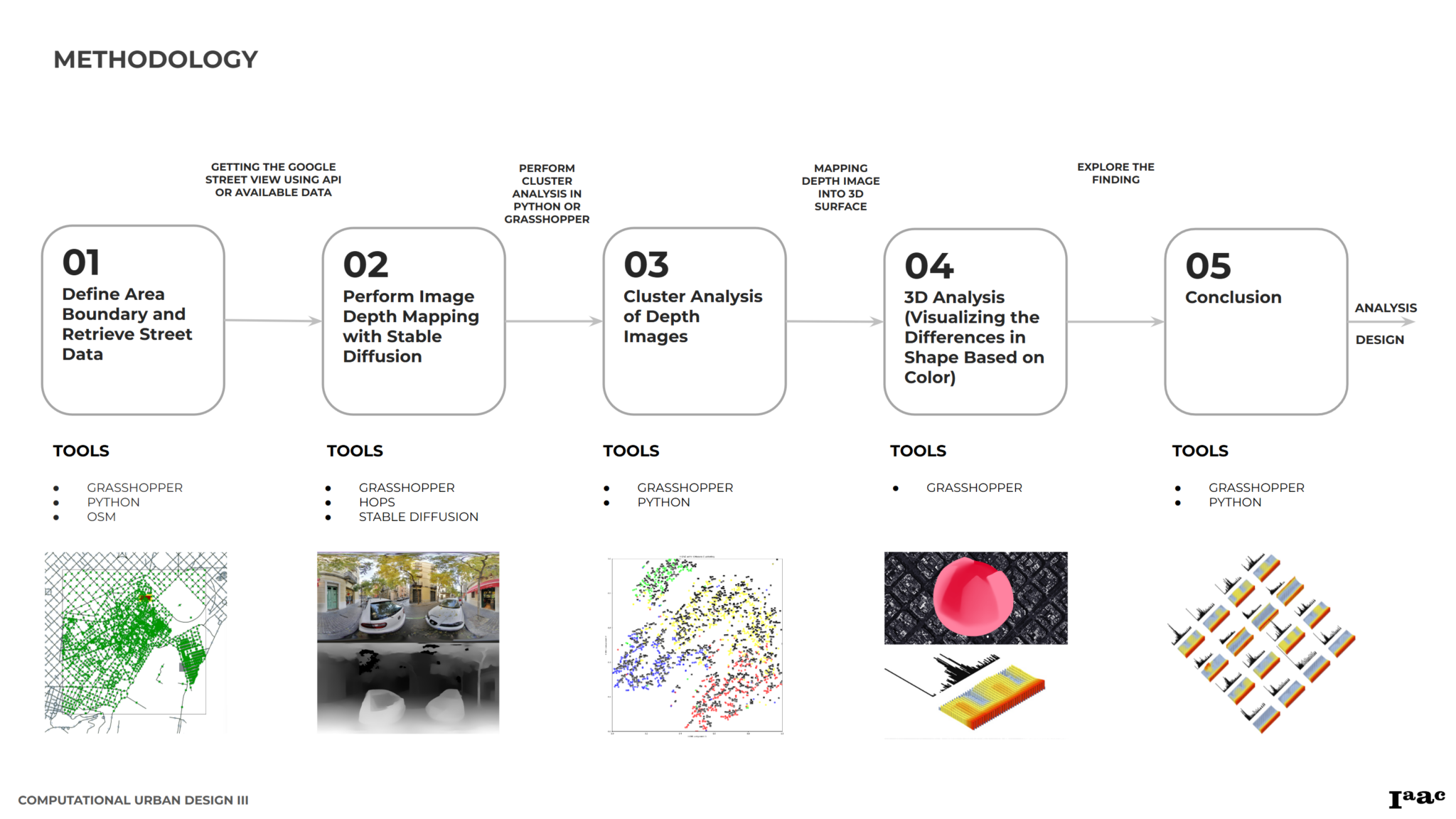
The pipeline stays explicit from image collection to analysis.

The methodology diagram makes the sequence legible: site definition, panorama gathering, depth transformation, clustering, and interpretation. Keeping this chain visible is what lets the project read as a coherent analytical system instead of a collage of outputs.

Reveal

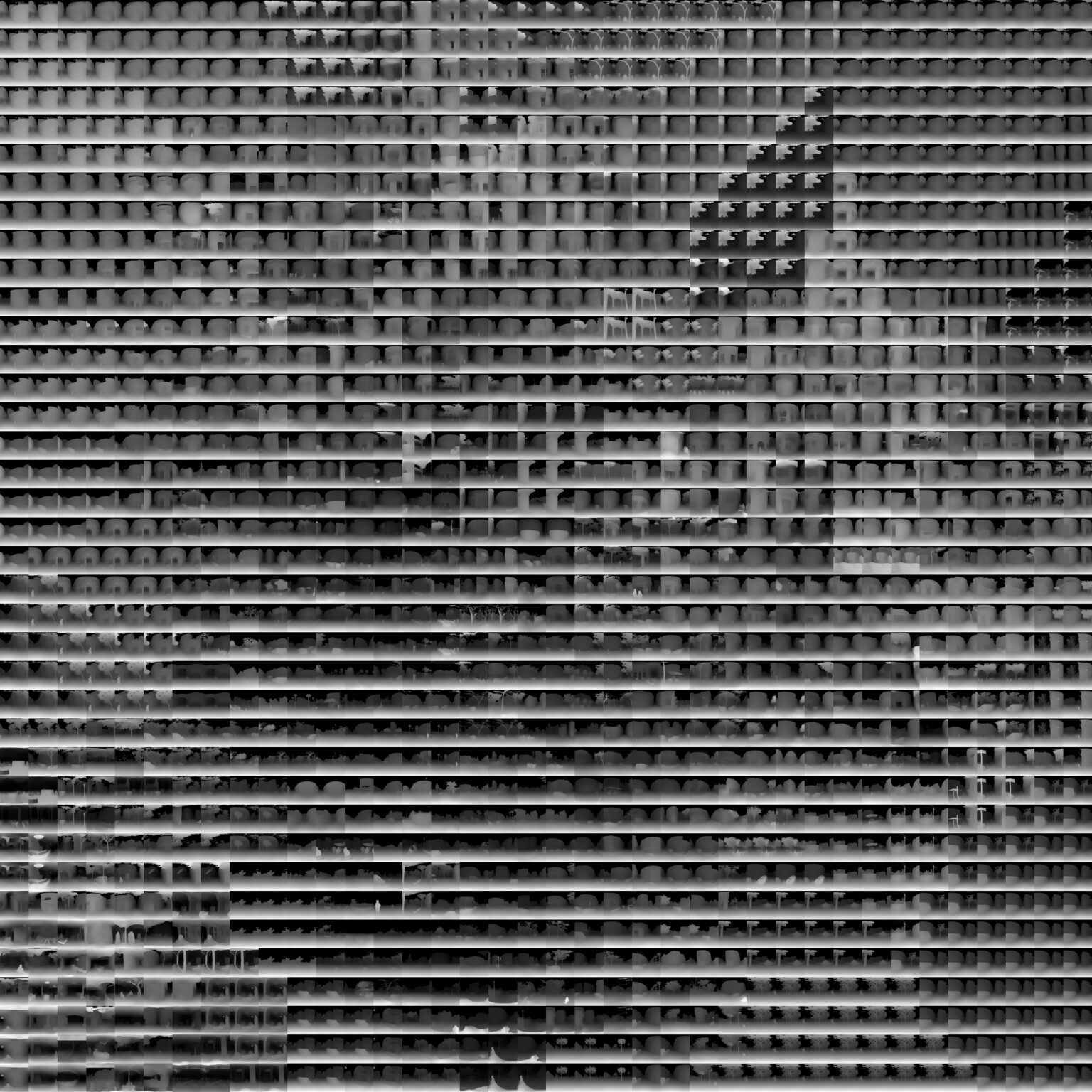
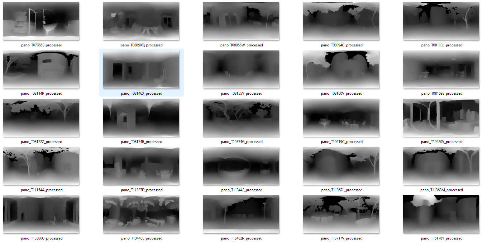
Stable Diffusion depth estimation converts texture into distance.

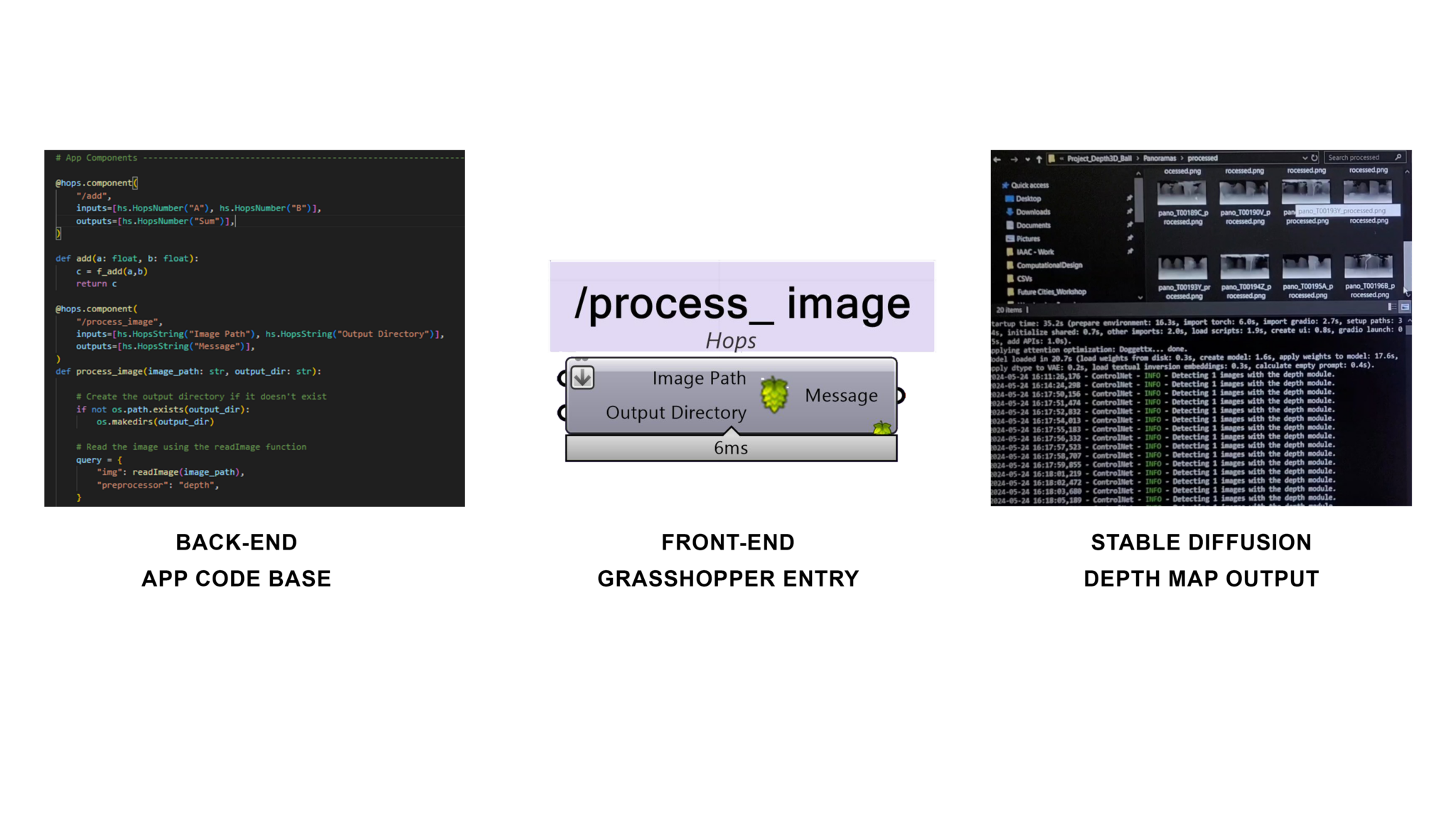
With the ControlNet Midas workflow, lighter pixels indicate nearer objects and darker values represent deeper space. The result is not a photorealistic reconstruction; it is a consistent distance proxy that can be compared from one panorama to another.

  • Near-field clutter becomes legible as bright, dense depth information.
  • Open or recessed spaces appear as darker, more distant fields.
4
Four linked stages keep the workflow interpretable.

Sampling, depth estimation, clustering, and reading each depend on the previous stage. Removing one collapses the story and the analytical usefulness of the page.

Act III

Clustering the urban field

Once each street view has been translated into a depth signature, the project can search for families of similar conditions rather than interpreting every scene by hand.

Feature extraction

Depth mapping changes what the model notices.

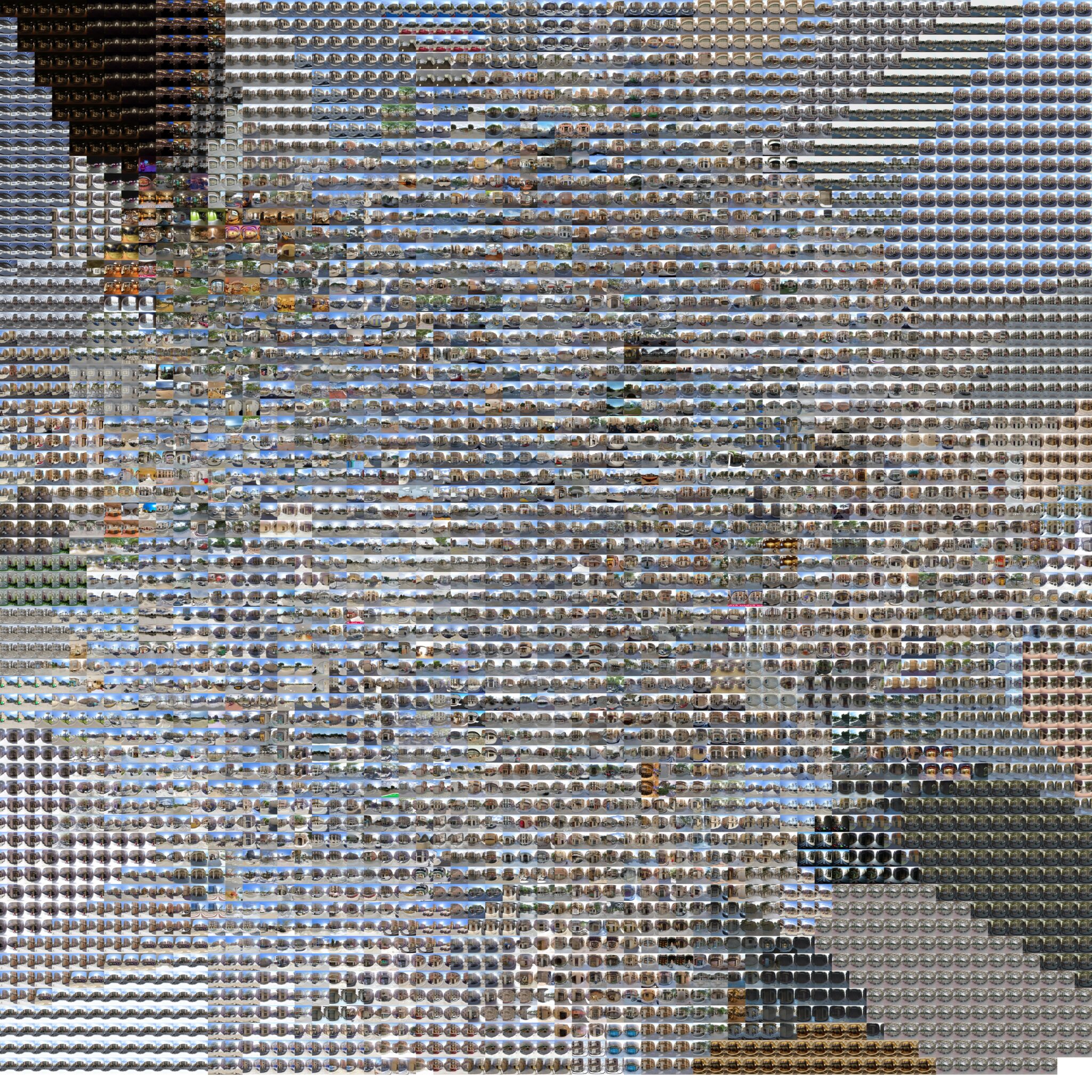
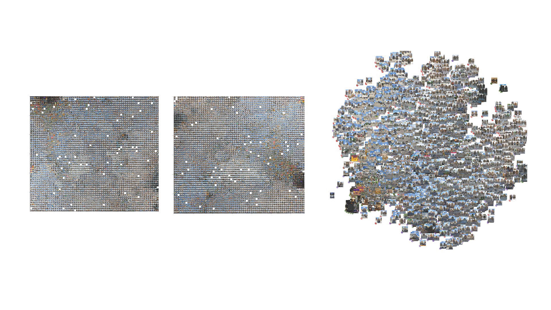
The side-by-side feature panels show the shift from appearance-driven similarity to geometry-driven similarity. That matters because the project is trying to read street conditions, not simply group images with similar colors or lighting.

t-SNE on panoramas

Original images still carry strong visual neighborhoods.

t-SNE helps compress high-dimensional imagery into a readable field, showing which panoramas share related visual traits. It becomes a first pass at city-scale pattern recognition.

t-SNE on depth

Depth clusters reveal spatial likeness across different scenes.

Running the same reduction on depth outputs exposes comparable street sections even when facades, materials, or weather conditions differ. The grouping is driven by distance structure rather than image surface.

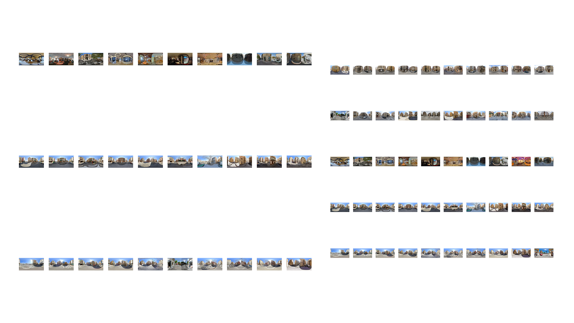
Directory output

Cluster folders turn model output into an operational urban atlas.

Saving clustered images into grouped directories makes the results usable by humans. The project does not stop at algorithmic output; it organizes the material so teams can inspect recurring street conditions and compare them across neighborhoods.

Act IV

Reading street quality

The resolution of the project is interpretive: using depth distributions and cluster differences to infer openness, enclosure, clutter, and the spatial character of a street.

Interpretation framework

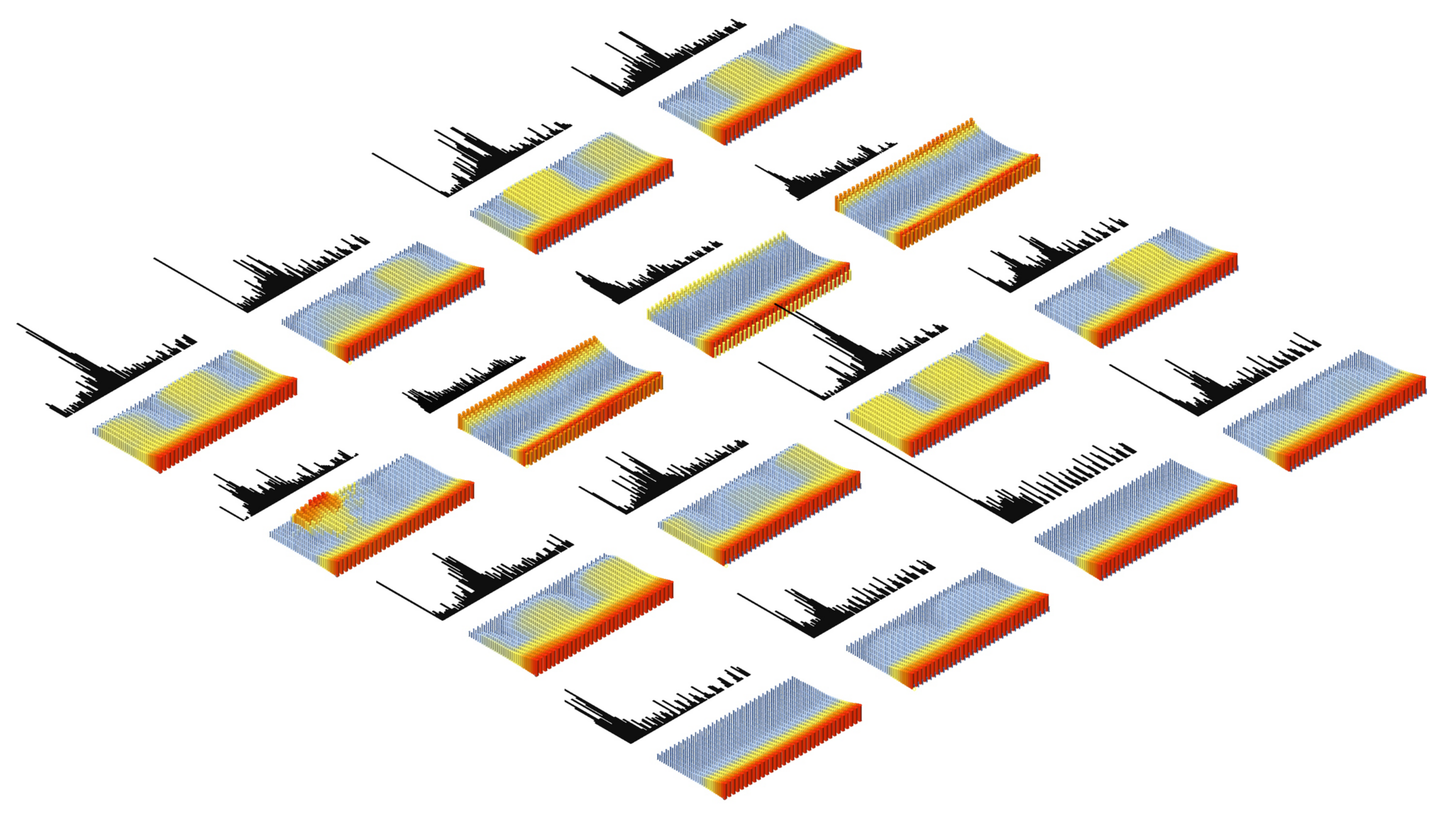
X-axis: where the street edge sits.

Depth value bins describe how close or distant the dominant scene elements are. Lower ranges hint at tight edges, nearby furniture, or close building fronts; longer ranges suggest wider setbacks, deeper vistas, and greater openness.

Y-axis: how often that condition appears.

Frequency indicates how consistently a depth condition repeats through the panorama. A dense count in short ranges can point to clutter or compression, while lower, more distributed values can indicate roomier pedestrian conditions.

Clusters become decision-support, not decoration.

Once grouped, similar streets can be compared as recurring urban types. That gives the workflow value for urban planning: it helps identify which neighborhoods share narrow, open, dense, or balanced street characteristics without auditing every street manually.

Analytical chart comparing 3D texturization and street distribution across clusters
Analytical reading The chart acts as the bridge from model output to urban interpretation, comparing how each cluster distributes near and far spatial readings.
Resolution

Three ways the project reads street quality.

The conclusion is not that one cluster is universally better. It is that different depth distributions point to different spatial conditions, each with implications for accessibility, comfort, openness, and street life.

Even distributions suggest balance.

When depth values spread more evenly, the street often reads as coherent and legible: setbacks, edge conditions, and furniture feel more consistent across the scene.

Short-range peaks suggest compression.

High counts near the camera can indicate narrow corridors, heavy furniture, or closely packed edges. That can mean lower pedestrian comfort, but it can also signal intense urban activity.

Long-range peaks suggest openness.

Higher counts at longer depths point toward wider streets, larger setbacks, or more open public space. The tradeoff is that openness can sometimes reduce street intensity.

Final Compliance

References and source logic

This version preserves the original project narrative in semantic HTML while rebuilding it as a paced scrollytelling case study. Motion is limited to narrative reveals and sticky image transitions, with reduced-motion fallbacks and local media throughout.

Core methods
  1. Study area definition using street geometries and coordinate-based selection.
  2. Panorama collection and mapping through Python and Grasshopper workflows.
  3. Depth translation using Stable Diffusion and ControlNet Midas.
  4. Dimensionality reduction and grouping with t-SNE and clustering analysis.